How an LNG Plant Works from Feed Gas to Ship Loading

Every stage of an LNG facility depends on what happened upstream. A pretreatment upset that lets even trace CO₂ through to the cryogenic section can freeze inside aluminum heat exchangers and shut down a liquefaction train. Typical specific energy consumption for LNG liquefaction sits around 280 kWh per tonne, yet well-run facilities consistently beat that number.

That gap comes down to operational discipline: understanding how each stage connects to the next, and where small upstream drifts turn into downstream energy and capacity losses.

TL;DR: How an LNG Plant Works from Feed Gas to Ship Loading

LNG production links pretreatment, liquefaction, storage, and export, where small upsets cascade quickly.

Liquefaction Consumes the Majority of Plant Energy

• The optimal mixed refrigerant blend shifts with feed composition, ambient temperature, and compressor condition. Static strategies leave capacity on the table.
• The binding constraint changes within a single day; operators often build conservatism into multiple setpoints simultaneously.

Ship Loading: Where Upstream Choices Become Visible

• Loading generates BOG surges that exceed steady-state rates by several multiples, pushing decisions back into tank pressure control and liquefaction rate.
• Each stage’s performance shapes what the next one has to manage. Without cross-stage visibility, operators end up managing their section in isolation while problems compound elsewhere.

The sections below trace the handoffs that determine energy performance across the full process chain.

Pretreatment: Where Small Drift Becomes a Downstream Shutdown

The pretreatment sequence protects the cryogenic section from contaminants that would destroy it: CO₂ and H₂S that solidify below −78°C, mercury that causes liquid metal embrittlement in aluminum heat exchangers, and moisture that forms ice at cryogenic temperatures. Mercury’s hard to catch because it can show up at parts-per-billion concentrations in feed gas and still cause catastrophic MCHE failure. Sulfur-impregnated carbon beds must maintain capacity throughout their lifecycle, and if breakthrough monitoring lapses, the first sign of a problem may be the MCHE itself.

Each stage protects the one downstream, and the sequence itself matters. Acid gas removal first prevents CO₂ from interfering with mercury adsorbents, and mercury removal before dehydration protects the path to cryogenic processing. Reversing any two stages risks equipment damage or specification exceedances that can take a liquefaction train offline.

Drift Shows Up in Leading Indicators, Not Final Specs

The operational risk in pretreatment is gradual drift that compounds across shifts, not a sudden failure. Solvent contamination and foaming push amine contactors toward higher differential pressure and lower mass transfer efficiency, showing up as gradual CO₂ slip long before a trip point is reached. Amine systems targeting CO₂ below 50 ppmv can lose that margin slowly enough that no single shift sees the trend. That’s why gas processing optimization depends on tracking these leading indicators continuously rather than waiting for final-spec alarms.

Dehydration units show a similar pattern: bed switching frequency and regeneration heater performance often tell the story before outlet moisture rises. Liquid carryover into molecular sieve beds causes permanent adsorbent damage, which means the early indicators of upstream separation quality are as important as the dehydration spec itself.

Keeping these leading indicators visible across shifts, rather than relying on final-spec alarms, is what prevents a pretreatment drift from becoming a liquefaction train trip. The challenge is that these signals live in different systems and different operators’ heads. Without a shared, data-first picture of current pretreatment health, consistent interpretation across shifts becomes difficult. When that visibility exists, each shift inherits not just setpoints but context about where the system is trending, and the kind of slow drift that costs a facility thousands of tonnes over a quarter gets caught in days instead of months.

Liquefaction Consumes the Majority of Plant Energy

Liquefaction cools treated gas from roughly 40°C to −160°C through staged refrigeration cycles, consuming more energy per tonne of LNG than any other process stage. In the widely deployed C3MR configuration, propane pre-cooling reduces gas temperature before the mixed refrigerant cycle takes over in the main cryogenic heat exchanger (MCHE). The MR blend is designed to match the natural gas cooling curve, but that match degrades as operating conditions shift.

Heat exchanger performance in the MCHE directly sets the ceiling on what the train can produce: fouling or maldistribution shows up as lost production before anything alarms.

Mixed Refrigerant Composition Control

Mixed refrigerant composition control is where operational skill meets thermodynamics. As feed gas composition shifts, as ambient temperature changes with seasons, as compressors age and lose efficiency, the optimal refrigerant blend changes too. In air-cooled systems, summer-to-winter swings can mean the difference between running at nameplate and running well below it.

These sensitivities make mixed refrigerant optimization an ongoing operations task, not something locked in at commissioning. Many facilities still manage it through periodic manual adjustments rather than continuous rebalancing.

Managing Shifting Constraints

One practical reason liquefaction optimization is difficult to “set and forget” is that the limiting constraint shifts within a single day. Sometimes the driver power limit is binding; at other times, compressor surge margin, refrigerant condenser approach temperature, or MCHE temperature approach becomes the first constraint reached. Operators often compensate by building conservatism into multiple setpoints at once, because pushing one constraint too hard can trigger recycling or instability that takes hours to unwind.

Traditional APC handles individual loops well, but it wasn’t designed to rebalance across the full constraint envelope as conditions shift. Consistent optimization depends on treating those constraints as a coordinated set rather than independent knobs, and on making constraint status visible so operators don’t rediscover the active limits from scratch at every shift change.

How well liquefaction runs also determines what the storage system has to manage: a train running at peak output fills tanks faster, generates more flash gas, and compresses the scheduling window before the next cargo.

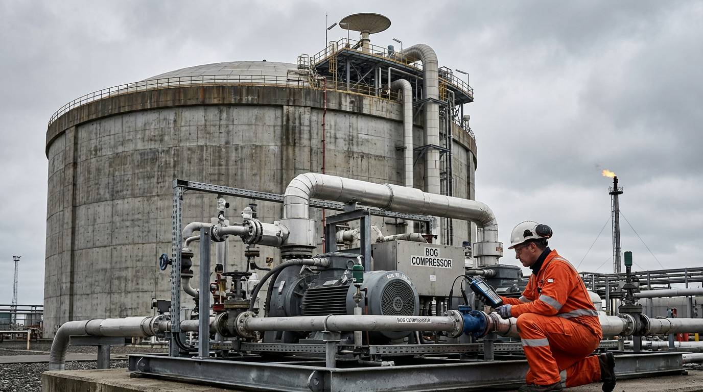
Storage and BOG: Equipment Rarely Sized for Everything at Once

Boil-off gas management equipment is sized for normal operations, not worst-case convergence. BOG compressors have stable operating windows and surge limits, recondenser capacity depends on available subcooled LNG, and fuel gas headers can absorb only so much incremental vapor without upsetting combustion controls.

Onshore storage tanks are typically designed to a BOG rate of around 0.05% per day of tank inventory under steady-state conditions, though actual rates vary with tank design, fill level, and ambient conditions. Reliquefaction preserves the most product value, but recondenser performance depends on having enough subcooled LNG flow, which ties BOG recovery directly back to liquefaction output and rundown temperature.

When reliquefaction capacity, fuel gas demand, and flare limits all tighten at the same time, operations has to choose between backing down liquefaction, changing tank circulation practices, or accepting higher flaring risk. Those trade-offs become more consequential as loading approaches.

Tank Pressure and Rollover Risk

Tank pressure adds its own constraints on top of BOG handling.

Thermal stratification, where warmer LNG layers sit above cooler ones, can lead to rollover events that release vapor volumes overwhelming normal BOG handling capacity within minutes. Detecting early stratification through temperature profile monitoring matters precisely because the consequences arrive faster than operators can react to them.

Keeping storage operations efficient means seeing these situations develop, not scrambling after a pressure excursion forces the issue. And that gets harder when the data operators need sits in separate systems: tank gauging in one place, BOG compressor status in another, loading schedule in a third.

Those decisions benefit from shared visibility into current storage conditions, BOG capacity, and the likely loading timeline, because ship loading is where all of these pressures converge at once.

Ship Loading: Where Upstream Choices Become Visible

Ship loading compresses every upstream trade-off into a single high-stakes window. A typical 170,000 m³ carrier requires roughly 12 hours of active loading, plus additional time for cooldown, line chilldown, and disconnection. Displaced vapor returns to shore through the vapor return system, but the volume can exceed steady-state BOG rates by several multiples. That pushes decisions back into tank pressure control and sometimes all the way upstream into liquefaction rate selection.

Loading is rarely a single steady rate from start to finish. Ramp-up limits protect loading arms and manage thermal stresses, while vapor return pressure constraints can force rate reductions mid-load. A rate change at the jetty shows up quickly as a different BOG load on shore. If storage pressure is already elevated, or if BOG compressors are running near capacity, that rate change cascades into decisions about liquefaction output, fuel gas balance, and flare management simultaneously.

Shift Handovers During Active Cargo

Complicating matters further, a 12-hour loading window often spans a shift change. The operator who began the load may not be the one managing the final topping-off and disconnection, and the reasoning behind earlier rate decisions can’t just live in one person’s head. During active loading, no single operator can track how liquefaction rate, storage pressure, BOG capacity, and vapor return limits all affect each other simultaneously.

When operators have visibility into how their decisions ripple upstream and downstream, and when AI optimization trained on actual plant operating history handles the cross-stage coordination continuously, the result is more consistent performance across shifts, seasons, and operating conditions. That kind of coordination is what turns a collection of self-optimizing unit operations into a facility that performs as a single integrated system.

Closing the Gap Across the Full Process Chain

For LNG operations leaders looking to close the gap between current performance and what their facility is capable of, Imubit’s Closed Loop AI Optimization solution learns from actual plant data across all process stages and writes optimal setpoints in real time through existing control infrastructure.

The platform delivers LNG production optimization by coordinating across the constraint envelope that shifts between pretreatment, liquefaction, storage, and export, so every shift works from the same optimized picture. Plants begin in advisory mode, where the system recommends setpoint changes and operators evaluate them against their own experience, building confidence before progressing toward closed loop operation at a pace that matches their organization’s readiness.

Get a Plant Assessment to discover how AI optimization can reduce specific energy consumption and improve coordination across your LNG facility’s process stages.

Frequently Asked Questions

Why is the sequence of pretreatment stages in an LNG plant so important?

Each pretreatment stage protects the one downstream. Acid gas removal prevents CO₂ and H₂S from solidifying in cryogenic equipment, mercury removal protects aluminum heat exchangers from embrittlement, and dehydration achieves the ultra-low moisture specification immediately before the cryogenic section. Reversing any two stages risks equipment damage or specification failures that can shut down a liquefaction train. Well-coordinated gas processing plants treat this sequence as a tightly coupled system, not independent unit operations.

How do ambient temperature changes affect LNG plant production capacity?

Ambient temperature directly impacts refrigeration efficiency because air-cooled systems reject heat to the surrounding environment. In cooler weather, refrigerant condensing temperatures drop, compressors operate more efficiently, and production can increase compared to peak summer conditions. Plants with seawater cooling see more stable year-round performance. Dynamic adjustment of refrigerant composition and compressor operating points captures seasonal capacity that static setpoints miss.

What makes BOG management during ship loading more complex than steady-state operations?

During steady-state operations, BOG systems primarily handle vapor generated by heat ingress into storage tanks. Ship loading adds a second, larger source: vapor displaced from the carrier’s cargo tanks as they fill with liquid. The combined vapor volume can exceed steady-state BOG rates by several multiples, requiring coordinated process control across liquefaction, storage levels, and vapor return line pressure simultaneously.